3. Functions

3.1. Basic functions

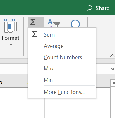
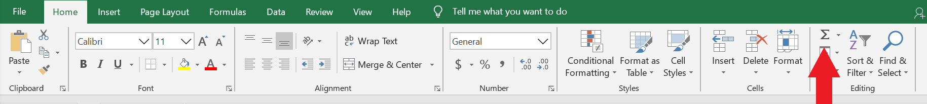
In the figure above, there are five basic functions:

1. Sum

2. Average

3. Count

4. Max

5. Min

3.1.1. Sum

The sum function adds a selection cells and takes on the following form:

=sum(number1,number2,number3,...)

There are three ways to go about using sum.

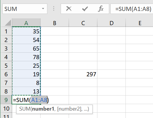
The first way is to manually type =sum(A1,A2,A3,A4,A5,A6,A7,A8) in a blank cell.

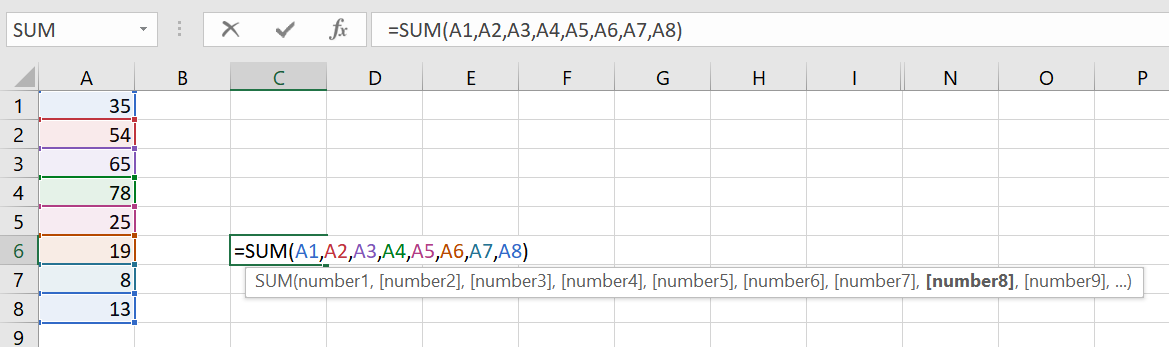
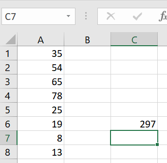
Excel automatically shows the function’s parameters underneath the =sum( to aid the user in finishing the formula. This helpful dialog box appears every time a function is in use. The results of the sum of the numbers are shown below.

The second way is to use the shortcut Alt+=.

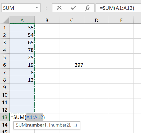
When using the Alt+= shortcut in the cells of the figures above, note that Excel automatically recommends the range of cells to add for the user. Observe one of major differences between method one and two. In the first method, we manually typed in each cell we wanted to calculate. In the second method, Excel uses a : to select the start of the sum range to the end of the sum range. The rest of this book will use a : when selecting a range of contiguous cells in a formula. 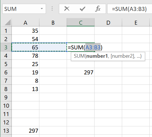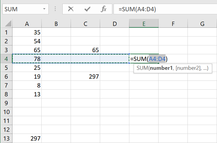The two figures below demonstrate using the Alt+= shortcut horizontally.

The third way is to click on the sigma button in the Editing section of the Home ribbon. Please note that doing this produces the same results as the second method above.

3.1.2. Average

The average function adds a selection of cells and then divides that sum by the number of cells it added. Below is the form of the average function. Notice that its form is the same as the sum function.

=average(number1,number2,number3,...)

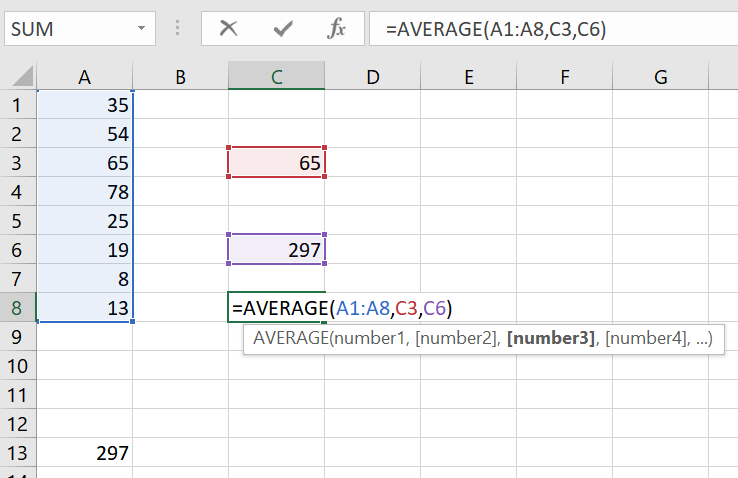
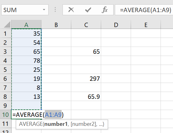
The average function does not have a shortcut. Thus, only methods 1 and 3 for sum function will work for the average function. Start by selecting the cell that will hold the average calculation and type =average(. Once that has been typed, select the cells that will be included in the calculation. To select cells that are not adjacent to one another, press the Ctrl button and click on the cells to be included in the calculation.

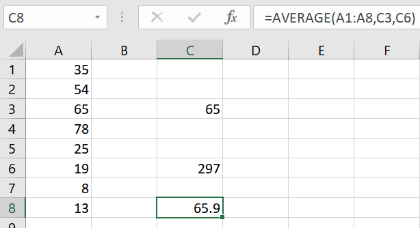
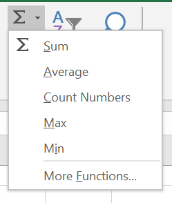
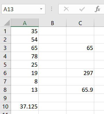
Using method three, select the cell that will hold the average calculation. Click on the down arrow to the right of the sigma button and select Average. Just like the sum function, Excel will recommend a range of cells to average. It should be noted that even though 9 cells are selected, it will only take the average of the 8 cells which contain numbers. It will not calculate the 9th cell.

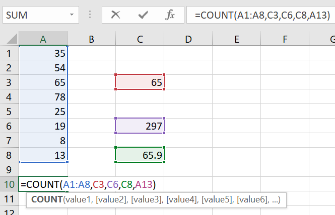
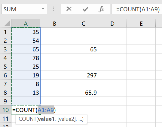
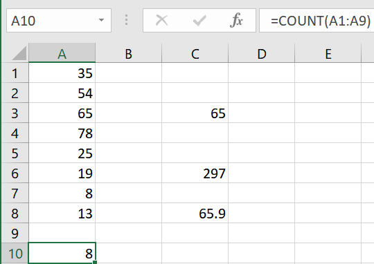
3.1.3. Count

The count function evaluates a selection of cells and counts how many of those cells contain numeric values. count, max, and min have forms just like the functions sum and average.

=count(value1,value2,...)

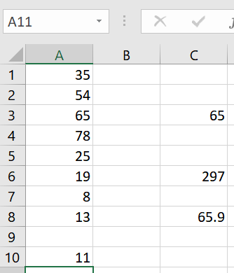
Using methods 1 and 3 above produces the following results:

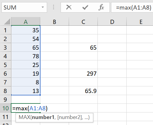
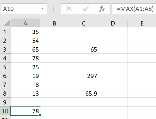
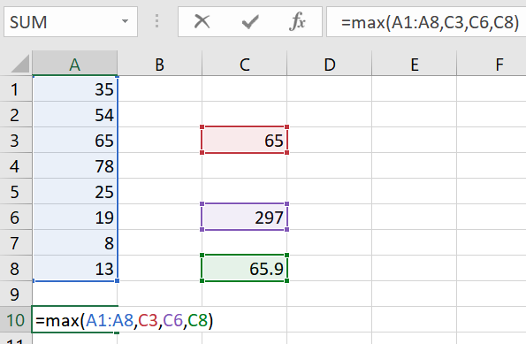
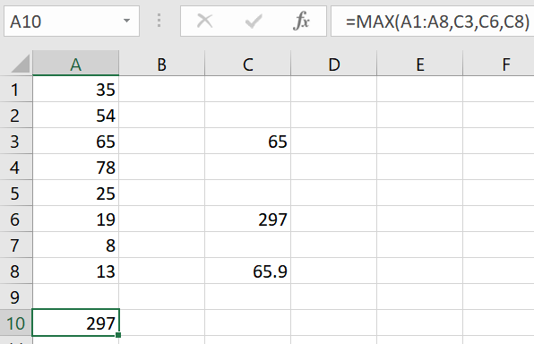
3.1.4. Max

The max function evaluates a selection of cells and returns the maximum numerical value of those cells.

=max(number1,number2,...)

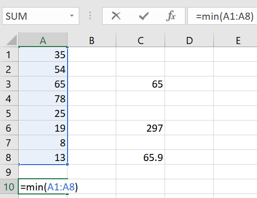
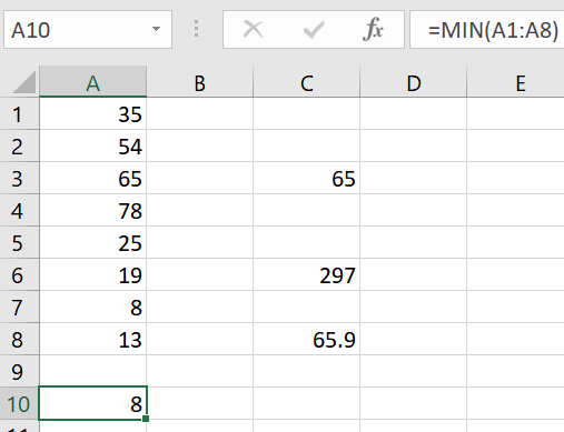
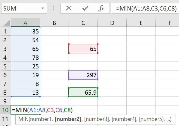
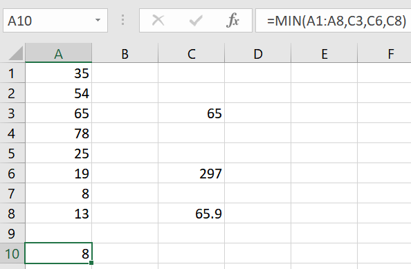
3.1.5. Min

The min function evaluates a selection of cells and returns the minimum numerical value of those cells.

=min(number1,number2,...)

3.2. Concatenate

concatenate joins data from various cells. There are two ways to concatenate data.

1. concatenate - takes the form of =concatenate(text1,text2,text3)

2. &

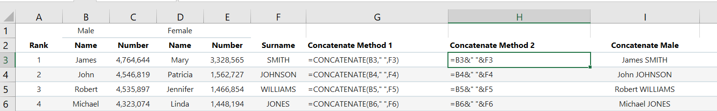
The figure below shows the joining of male first names, column B, with a space and surnames, column F. Observe that column G (method 1) and column H (method 2) both produce the same result in column I.

3.3. Left, Mid, Right

The left, mid, and right functions extract information from text or a cell. left starts at the left most character and returns the specified number of characters to the right. right does the opposite. right starts at the right most character and returns the specified number of characters to the left. mid is slightly different. it takes on three parameters: text, start_num, and num_chars. After specifying the text to be extracted, a starting character position in the text or cell is chosen, and then the specified number of characters to the right of that starting position is returned.

1. left takes on the form =left(text,num_chars)

2. mid takes on the form =mid(text,start_num,num_chars)

3. right takes on the form =right(text,num_chars)

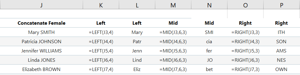
The text in each of the functions above can be a string like superior or it can be a cell like in the figure below. The left function returns the 4 left most characters. The right function returns the 3 right most characters. The mid function starts at the 6th character in the string and returns the 3 characters to the right of the 6th character. These functions are great for parsing information from cells that have uniform values.

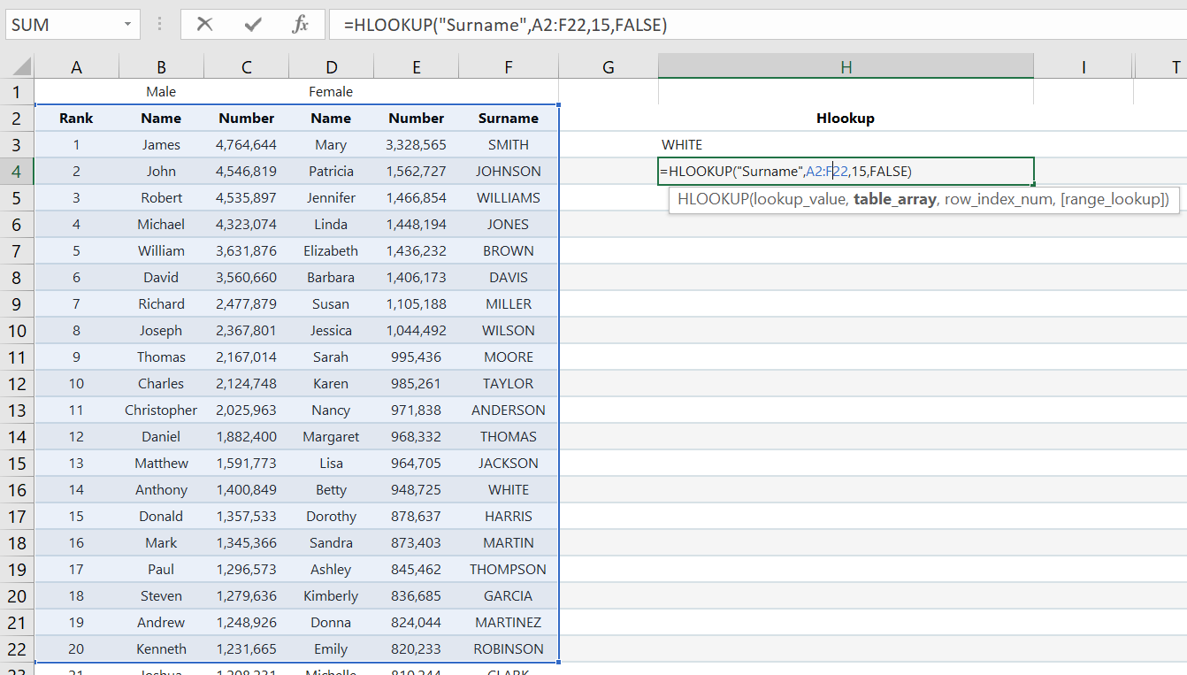
3.4. Hlookup

hlookup (horizontal lookup) is a function that retrieves data from a specific row in a table. The function has the following form:

=hlookup(value,table,row_index,[range_lookup])

In the example below, the value is Surname, the table is starts from A2 and spans to F22. The row_index is 15 and the range_lookup is False. hlookup needs the 2nd row to search for the value Surname. Once it finds that value, it will count down 15 rows from the second row and grab the value at that row. Observe that the Surname of the row 15 is actually the 14th ranked surname and not the 15th ranked surname which is Harris. If the 15th ranked surname was desired, then the row_index should be 16 and not 15.

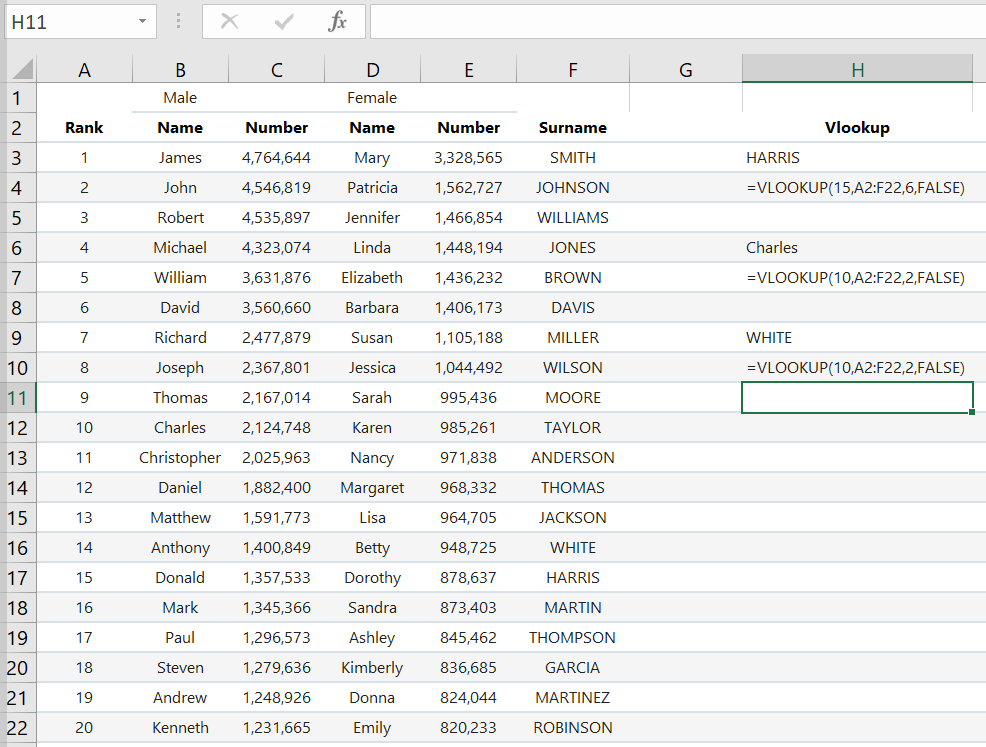
3.5. Vlookup

vlookup (vertical lookup) is like hlookup except that it retrieves the data from a specific column. Its form is the same as hlookup and is listed below:

=vlookup(value,table,row_index,[range_lookup])

In the example below, row H9 and H10 is the vlookup method to obtaining the same result as the hlookup example that was just shown above. Just like row 2 was the first row in hlookup, the first column for vlookup is column A. In cell H3 and H4, vlookup returns for the 15th ranked surname. While in cells H6 and H7, vlookup returns the 10th ranked male name.