6. Conditional Formatting

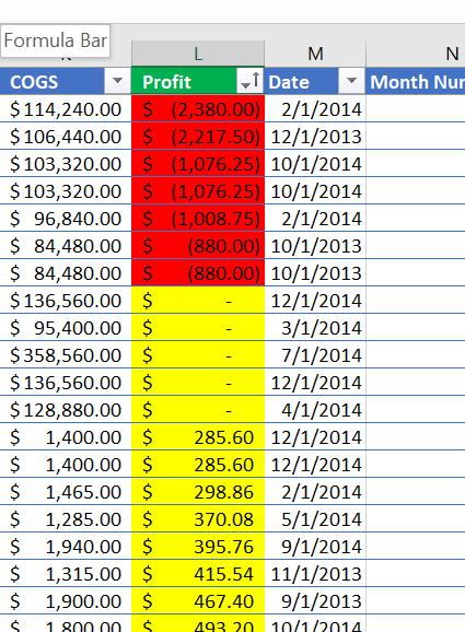
Conditional formatting allows users to highlight their spreadsheet based on criteria. For example, highlight a cell red if its value is less than zero. Or, highlight a row if a value in one cell in that row contains a specific value. Multiple conditions can be placed on one cell. The cell can be highlighted red if the value is less than zero. If the cell is in between 0 and 50, it will be highlighted yellow. Or, if it is greater than 50, it will be highlighted green.

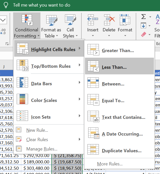
Using the same financial sheet, conditional formatting will be placed on certain columns to illustrate its capabilities. First, highlight the Profit column by clicking on the letter L. Then, on the Home ribbon, click on Conditional Formatting, hover the mouse arrow on Highlight Cells Rules and click on Less than.... A Less Than dialog box will popup. Enter 0 into the left box. Click on the down arrow to the right of Light Red Fill with Dark Red Text to get a drop down.

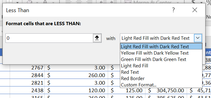
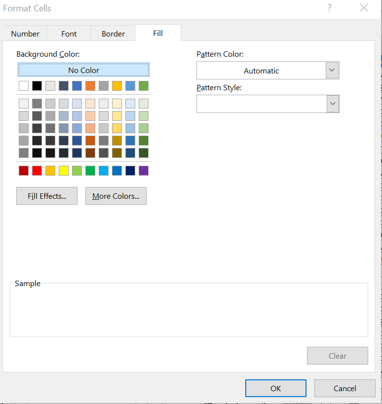
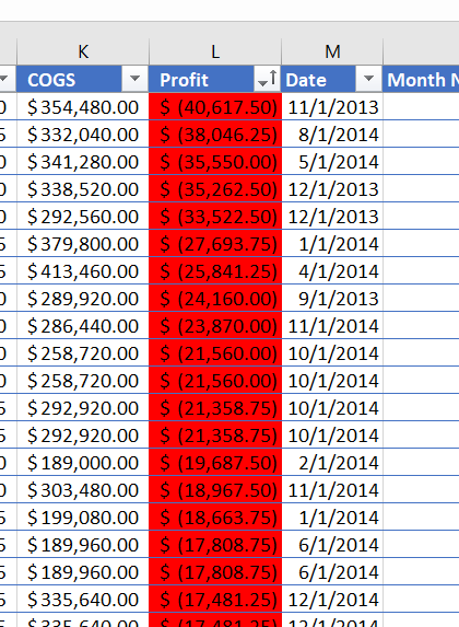
A preset set list of options will be available or Custom Format... can be selected. Click on Custom Format... and a Format Cells dialog box will popup. Select the second from the left red color and click Ok. Observe that values less than 0 in that column are already highlighted red. Click Ok again to apply the changes.

Click on Conditional Formatting, hover the mouse arrow on Highlight Cells Rules and click on Between.... In the Between dialog box, enter 0 into the left fill-in and 50000 into the middle fill-in box. Next, click the right drop-down box and click on Custom Format. Select the Yellow color on the Format Cells and click Ok in both the Format Cells and Between dialog boxes.

Repeat the same steps above except choose Greater Than..., enter 50000 in the Greater Than left fill-in box, and the color Green. Scroll down the spreadsheet and observe the colors of the cells of the Profit column.

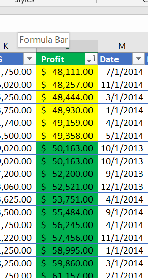
Experiment with various columns and options for conditional formatting to see how each options visually changes the spreadsheet.